Section 3.2 - Polynomial Functions

Let $n$ be a non-negative integer. Then a polynomial of degree $n$ is a function of the form

$$p(x) = a_n x^n + a_{n-1} x^{n-1} + \dots + a_2 x^2 + a_1 x + a_0$$

• In the above definition, $a_n\neq 0$ is called the leading coefficient. The remaining coefficients are all permitted to be equal to $0$, but if $a_n=0$ then the polynomial does not have degree $n$. The coefficient $a_0$ is called the constant term.

• Constant functions, linear functions, and quadratic functions are all examples of polynomials (of degrees $0$, $1$, and $2$ respectively).

• The domain of every polynomial is all real numbers.

• The sum, difference, product, and composition of any two polynomials is another polynomial. The quotient of two polynomials is a rational function, which we will study in section 3.4.

The symmetry of the graph of a polynomial is determined by the parity of the degrees of its terms.

• A polynomial is odd when each term has odd degree and even when each term has even degree. For example $p(x) = 2x^5 + 5x^3 - 7x$ is an odd function while $q(x) = 3x^4 - 7x^2 + 11$ is an even function. Notice that the coefficients have nothing to do with the function’s symmetry.

• A polynomial which has terms with both even and odd degrees is neither an even function nor an odd function. For example $r(x) = x^2 - x$ is neither even nor odd.

We’ve already studied the graphs of $y= x^0 = 1$ and $y = x$. For the remaining integer powers of $x$ it helps to break them up by pairity. First we examine even powers of $x$, then odd powers.

• 

• 

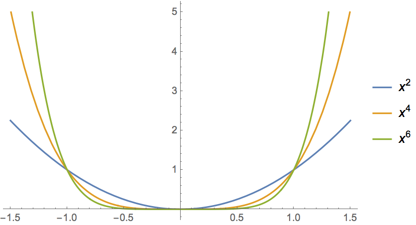
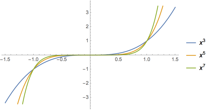
There are a few things to notice here.

• Firstly, all of the graphs contain the point $(1,1)$. All the graphs of even powers contain the point $(-1,1)$ and the graphs of odd powers contain the point $(-1,-1)$.

• The end behavior is determined by the pairity of the exponent. If $n$ is even, then $f(x)=x^n\to\infty$ as $x\to\pm\infty$. If $n$ is odd, then $f(x)=x^n\to\infty$ as $x\to\infty$ and $f(x)\to-\infty$ as $x\to-\infty$.

• Inside the interval $(-1,1)$ the graph of $y=x^n$ gets flatter as $n$ gets larger. Outside that interval, the graph gets steeper for larger $n$.

It turns out that the end behavior of every polynomial is determined by the leading term. For instance, consider the polynomial $p(x) = -2x^4+x^2-4x+1$. The leading term is $-2x^4$, and so $p(x)$ has the same end behavior as $q(x)=-2x^4$. We can see that $q(x)$ is a vertical stretch and reflection of $y = x^4$, so $q(x)\to-\infty$ as $x\to\pm\infty$.

If $f$ is any function and $f(c)=0$, then $c$ is called a zero of the function. As we shall see, the zeros of a polynomial are very important. It turns out that $c$ is a zero of the polynomial $p(x)$ if and only if $x-c$ is a factor of $p(x)$. If $c$ is a zero of $p(x)$ and $n$ is the largest integer such that $(x-c)^n$ is a factor of $p(x)$ then we say $c$ is a zero of multiplicity $n$. The multiplicity of a zero determines the behavior of a graph near that zero. A zero of multiplicity $1$ is called a simple zero.

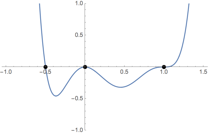
In the above picture there is a simple zero at $x=-0.5$, a zero of even multiplicity at $x=0$, and a zero of odd multiplicity at $x=1$.

• At a simple zero, the graph of a polynomial crosses the $x$-axis in much the same way that a line would.

• At a zero of even multiplicity, the graph of a polynomial flattens out and touches the $x$-axis, but remains on the same side.

• At a zero of odd multiplicity, the graph of a polynomial flattens out and crosses the $x$-axis.

Together, the leading coefficient and the zeros with their multiplicities completely determine the graph of a polynomial. We will formalize this notion in the next section.

The graphs of polynomials can be transformed according to the rules that we learned in chapter 2. For example, if we have the graph of $y = f(x) = x^4$, then we can determine the graph of $y = g(x) = -(x-3)^4$ (by shifting to the right by $3$ and reflecting about the $x$-axis).

Polynomials are good examples of what we call continuous functions. There is a useful theorem about such functions called the Intermediate Value Theorem. This theorem is very helpful in approximating the zeros of a polynomial that is not easy to factor.

• The Intermediate Value Theorem says that if $f$ is continuous on $[a,b]$ and $k$ is any number between $f(a)$ and $f(b)$ then $f(c)=k$ for some $c$ between $a$ and $b$.

For example, consider the polynomial $p(x) = x^4-2x-2$. The zeros are quite complicated and difficult to find, but we can approximate them very accurately using the Intermediate Value Theorem. Notice that $f(1) = 1-2-2=-3$ and $f(2) = 16-4-2=10$. Since $0$ is between $f(1)$ and $f(2)$, $f$ must have a zero between $1$ and $2$. Since $f(1.5)=.0625$ there must be a zero between $1$ and $1.5$. Since $f(1.4)\approx-0.96$ there must be a zero between $1.4$ and $1.5$. Every time we evaluate $f$, we get a smaller (and therefore more accurate) interval for the zero we’re seeking.